Exercise 7, Problem 8

Transform the estimates from problem 7 to world coordinates(by transforming the estimates, not the original scancoordinates).

 For this we need a function to transform the (alfa , r) pair from robot coordonates to world coordonates. After some easy geometry:

function result = robot2wrldLSQ(lsq,scannerPose)

alphaW = lsq(1)+scannerPose(3);

theRest = scannerPose(1)*cos(alphaW)+scannerPose(2)*sin(alphaW);

rW = lsq(2) + theRest;

result = [alphaW rW];

end

The difference is visible in scanPose2 where the two pairs differ.
This small change has been made to the code:

estimated11 = lsqline(line1) % in robot coords

estimated1 = robot2wrldLSQ(estimated11,scannerPose) %world coords

line1 = lsr2wrld(line1,scannerPose); %the scanned points in world coords (for a better plotting)

plot(...);

The result is:

estimatedn =    alpha      r 
estimated1 =    1.5708    1.0000
estimated2 =   -1.5708    1.0000
estimated4 =    0.0000    5.0000

It can be seen that the robot only scanned 3 different (colored) lines from point (3,0), facing angle 0 rad. But the LSQ lines are represented from the origo.
Also, the algorithm only displays estimated LSQs only for the lines 1, 2 and 4.

Compare estimates to the estimates from problem 6.

After running the algorithm for scannerPose1 we got the two set of estimates:

estimatednn =    alpha      r   - estimate of robot coords
estimatedn   =    alpha      r  - estimate of worlds coords
estimated11 =    1.5708    1.0000
estimated1   =    1.5708    1.0000
estimated22 =   -1.5708    1.0000
estimated2   =   -1.5708    1.0000

We can conclude that the algorithm works as intended.

Exercise 7, Problem 7

Same as problem 6 with scan2 (estimates in scanner coordinates).

The code is the same with the precedent problem with a small twik, which was revealed by not having the robot in the (0,0) point which coincidences with the robot's position in the robot coordinates.

y1 = 1 - scannerPose(2);
y2 = -1 - scannerPose(2);
x3 = 4 - scannerPose(1);
x4 = 5 - scannerPose(1);
scannerPose=[0 0 0]; % (0,0) because we are using robot coord

The results are:

estimatedn =    alpha      r
estimated1 =    1.5708    1.0000
estimated2 =   -1.5708    1.0000
estimated4 =   -0.0000    2.0000

Exercise 7, Problem 6

Find the points that belong to each of the three lines in scan1from problem 4
manually.

We know that for each line n we have the xn, yn, where n=1..4:
y1 = 1;
y2 = -1;
x3 = 4;
x4 = 5;

For finding the lines we have segmented the points from the scanner (Cartesian form) as belonging to one of the 4 lines:

line1=zeros(2,1); %first the lines are initialized
line2=zeros(2,1);
line3=zeros(2,1);
line4=zeros(2,1);
useScan = carthScan1; %we tell which set of points to use
for i=1:length(useScan)
   if    (useScan(2,i) == y1)
       line1 = [line1 useScan(:,i)];
   elseif(useScan(2,i) == y2)
       line2 = [line2 useScan(:,i)];
   elseif(useScan(1,i) == x3)
       line3 = [line3 useScan(:,i)];
   elseif(useScan(1,i) == x4)
       line4 = [line4 useScan(:,i)];
   end
end
Use the lsqline function to estimate the line parameters.

The code is the same as in Problem 5, with only the lines modified. The results are:

estimatedn =    alpha      r
estimated1 =    1.5708    1.0000
estimated2 =   -1.5708    1.0000

Exercise 7, Problem 5

Make a function line=lsqline(points) that outputs the estimated (alfa, r) for the line.

%% lsqline.m

function line = lsqline(points) %returns (alpha, r) from a set of points
Xs = points(1,:);
Ys = points(2,:);
sumXs = sum(Xs);
sumYs = sum(Ys);
sumXY = Xs*Ys';
lgnth = length(Xs);
sumXsq = Xs * Xs';
sumYsq = Ys * Ys';
alpha = 0.5 * atan2( (2*sumXs*sumYs-2*lgnth*sumXY) , (sumXs^2-sumYs^2-lgnth*sumXsq+lgnth*sumYsq) );
rsX = (1/lgnth) * sumXs;
rsY = (1/lgnth) * sumYs;
r = rsX*cos(alpha) + rsY*sin(alpha);
if r < 0
    r = -1 * r;
    alpha = alpha - sign(alpha) * pi;
end
line = [alpha r];
end

Testing with the lines x=5, y=3, x+y+3=0:

scannerPose = [0 0 0];
y1 = -10:1:10; x1 =  x1*0+5;
x2 = -10:1:10; y2 =  x2*0+3;
x3 = -10:1:10; y3 = -x3-3;
line1 = cat(1,x1,y1);
line2 = cat(1,x2,y2);
line3 = cat(1,x3,y3);
estimated1 = lsqline(line1)
estimated2 = lsqline(line2)
estimated3 = lsqline(line3)
figure(6);hold on;title('Exercise 7 Problem 5')
plot(line1(1,:),line1(2,:),'o', [scannerPose(1) estimated1(2)*cos(estimated1(1))],[scannerPose(2) estimated1(2)*sin(estimated1(1))],'LineWidth',2,'Color','m');
plot(line2(1,:),line2(2,:),'o', [scannerPose(1) estimated2(2)*cos(estimated2(1))],[scannerPose(2) estimated2(2)*sin(estimated2(1))],'LineWidth',2,'Color','b');
plot(line3(1,:),line3(2,:),'o', [scannerPose(1) estimated3(2)*cos(estimated3(1))],[scannerPose(2) estimated3(2)*sin(estimated3(1))],'LineWidth',2,'Color','r');
grid on; axis equal; axis tight;

estimatedx =    alpha      r
estimated1 =     0           5
estimated2 =    1.5708    3.0000
estimated3 =   -2.3562    2.1213

Exercise 7, Problem 3 and 4

Make a function transform(systempose_w, pos_l) that implements the transformation.

lsr2wrld.m

function wrld =  lsr2wrld(lsr, pose)
    tm = [cos(pose(3)) -sin(pose(3)); sin(pose(3)) cos(pose(3))]; %transf matrix
    wrld = lsr;
    for i = 1:size(lsr,2)
        wrld(:,i) = tm * lsr(:,i) + [pose(1); pose(2)];
    end
end

Make a 'lines' environment with the lines: [(0,1) (4,1)] [(4, 1) (4,5)] [(0,-1) (5,-1)] [(5, -1) (5,5)]

lines=[0 1 4 1; 4 1 4 5; 0 -1 5 -1; 5 -1 5 5]';

Take three scans with the laser poses (0,0,0), (3,0,0) and (4.5,0,pi/2).


scannerPose1 = [0 0 0]; %theta is in radians
scannerPose2 = [3 0 0]; %theta is in radians
scannerPose3 = [4.5 0 pi/2]; %theta is in radians

Convert the scans to world coordinates and plot the three scans in the same plot.

laserScan = laserscan2011(scannerPose1(1), scannerPose1(2), scannerPose1(3), lines, maxDist,resol,field_of_view);
carthScan1 = polar2carth(laserScan);
worldScan1 = lsr2wrld(carthScan1,scannerPose1);

laserScan = laserscan2011(scannerPose2(1), scannerPose2(2), scannerPose2(3), lines, maxDist,resol,field_of_view);
carthScan2 = polar2carth(laserScan);
worldScan2 = lsr2wrld(carthScan2,scannerPose2);

laserScan = laserscan2011(scannerPose3(1), scannerPose3(2), scannerPose3(3), lines, maxDist,resol,field_of_view);
carthScan3 = polar2carth(laserScan);
worldScan3 = lsr2wrld(carthScan3,scannerPose3);

hold on
figure(1);
hold on
plot(worldScan1(1,:),worldScan1(2,:),'bd')
plot(worldScan2(1,:),worldScan2(2,:),'mo')
plot(worldScan3(1,:),worldScan3(2,:),'kx')
legend('Pose 1 (  0 ,0)','Pose 2 (  3 ,0)','Pose 3 (4.5,0)');

Exercise 7, Problem 2

Make a function polar2carth(pol) that converts the polar coordinates in pol (same format as the Problem 1) to Cartesian coordinates x,y.

polar2carth.m

function carthScan = polar2carth (polarScan)
carthScan(1,:) = polarScan(2,:).*cos(polarScan(1,:));
carthScan(2,:) = polarScan(2,:).*sin(polarScan(1,:));

exercise7.m

carthScan = polar2carth(laserScan);
figure(2);
plot(carthScan(1,:),carthScan(2,:),'.')
title('Ex 7, Problem 2')

Exercise 7, Problem 1

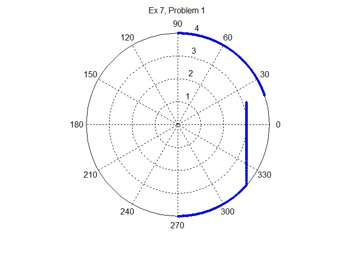
Make a 'lines' array with start point (3,-4) and end point( 3,1). Make a scan with scannerpose (0,0,0), maxDistance=4, resol=0.36 and field_of_view 180 and plot with the 'polar' function.

lines=[3 -4 3 1]';
scannerPose = [0 0 0]; %theta is in radians
maxDist = 4;
resol = 0.36;
field_of_view = 180;
laserScan = laserscan2011(scannerPose(1), scannerPose(2), scannerPose(3), lines, maxDist,resol,field_of_view);
figure(1);
polar(laserScan(1,:),laserScan(2,:),'.')
title('Ex 7, Problem 1')