Exercise 3, Problem 11

The two previous functions were used repeatedly to simulate the movement of the robot in the required patterns.
As in previous problems, we used the graphical implementation to show the results. Here they are:

As seen in the last figure, the program allows the robot to rotate in both directions.

Exercise 3, Problem 10

The function for rotation has the following form:


function move = turn(angle,speed)
   global robotpar ts pose;

   d = robotpar(1);
   size = round(abs(angle)*d/(2*speed*ts));   %size of the array
   array = zeros(size,3);                                 %initializing the array

   M = [            0;
                        0;
        (angle/abs(angle))*2*speed/d];
  
   for i=1:size
       th = pose(3);
  
       Rinv = [cos(th) -sin(th)  0;
                    sin(th)  cos(th)  0;
                       0          0       1];
      
       array(i,:) = pose' + Rinv*M*ts;
       pose = array(i,:);
   end  
   move = array;
end

As in the previous problem, both positive and negative values for the angles can be given.

Exercise 3, Problem 9

The function has the following form:


function move = forward(distance,speed)
   global ts pose;
   size = round(abs(distance)/(speed*ts));   %size of the array
   array = zeros(size,3);                              %initializing the array
   th = pose(3);

   Rinv = [cos(th)  -sin(th)  0;
               sin(th)    cos(th)  0;
                   0           0       1];
    
   M = [(distance/abs(distance))*speed;
                                0;
                                0];
    
   for i=1:size
       array(i,:) = pose' + Rinv*M*ts;
       pose = array(i,:);
   end

   move = array;
end

Both positive and negative values can be given for the distance and are correctly interpreted. The sign is taken into consideration when building the M array.

Exercise 3, Problem 8

The function was used in the following program:

T = 5;                                            % interval of time
ts = 0.01
pose = [0 0 0];                              % initial position
robotpar = [0.26 0.035 0.035];
wheelspeed = [5.714 5.714]
size = round(T/ts);                       % size of the array
array = zeros(size,3);                   % initializing the array
hold on;

for i=1:size
     array(i,:) = kinupdate(pose,robotpar,ts,wheelspeed); 
     a=[array(i,1) array(i,1)+0.5*cos(array(i,3))];
     b=[array(i,2) array(i,2)+0.5*sin(array(i,3))];
     line(a,b)
     pose = array(i,:);
end

array
xlabel('x [m]');
ylabel('y [m]');
plot(array(:,1),array(:,2),'Color','red','LineWidth',3);


The above program used the values from the first test. Both tests were performed and, in order to have a better understanding of the results, we implemented a graphical interpretation . The red line represents the trajectory of the robot and the blue line represents the orientation.


Test 1: The robot moves on a straight line on the OX axis.

 Test 2: Since the robot moves along its centre point, only its orientation changes and thus only the blue line can be seen.

Exercise 3, Problem 7

The function to calculate the next pose implemented in MATLAB has the following form:

function newpose = kinupdate(pose,robotpar,ts,wheelspeed)
th = pose(3);

Rinv = [cos(th) -sin(th) 0;

        sin(th) cos(th)  0;

         0        0      1];

d = robotpar(1);
rR = robotpar(2);
rL = robotpar(3);
phiR = wheelspeed(1);
phiL = wheelspeed(2);

M = [(rR*phiR+rL*phiL)/2; 
             0; 
     (rR*phiR-rL*phiL)/d];

newpose = pose' + Rinv*M*ts;

end

Where:
th = angle theta
d = distance between the wheels
rR and rL = the diameters of the right and left wheels
ts = sample time

phiR and phiL = the angular velocities of the left and right wheels 

Exercise 3, Problem 6

Taking the constraints from the previous problems we obtain the following matrix:

By extracting ξ from the equation we obtain:

Exercise 3, Problems 5.

Reducing the number of constraint equations to three:

Wheel 1, Rolling. Not constrained.
Wheel 2, Rolling. Not constrained
Wheel 3, Rolling. Constraint no.1.

Wheel 1, Sliding. Constraint no.2.
Wheel 2, Sliding. Identical to Wheel 1, Sliding.
Wheel 3, Sliding. Constraint no.3.

Exercise 3, Problems 3 & 4.

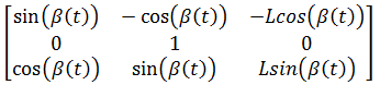
For problems 3 and 4 we have changed α, β and l accordingly and supplied the results.

Right wheel (wheel 2) constraints (rolling, sliding):

Front wheel (wheel 3) constraints (rolling, sliding):

Exercise 3, Problem 2. Constraints.

1) Rolling and sliding constraints for the left wheel (wheel 1):

2) Putting the equations into Maple (regarding α, β and l from Problem 1):

3) Querying the results / constraint matrices:

Exercise 3, Problem 1.

Finding α, β and l (from length) for the three wheels.

Wheel 1, Left (back): [π/2  0  w/2]'
Wheel 2, Right (back): [-π/2  π  w/2]'
Wheel 3, Middle (front): [0  β(t)   L]'

Note: for the right wheel, β is π because, when α is applied, it runs backwards; thus it must be turned another 180 deg (π rad);

Tricycle kinematics.

Figure 1 shows the wheel configuration of a tricycle with front wheel traction:

On this model, an introduction to kinematics is going to be applied through a series of steps.
These steps are the Problems in the next posts.